Confidence Intervals

What does it mean by 95% confidence interval?  This is something related to the Type I error and, therefore, the $\alpha$. If we set the $\alpha$ to 0.05, the confidence interval is (1-$\alpha$)*100 %. The 95% is the area under a distribution curve (0.95), between $z_{\alpha/2}$ and $1- z_{\alpha/2}$.

>> z2=norminv(0.025,0,1)
z2 =
   -1.9600
>> normspec([z2,-z2],0,1)
ans =
    0.9500

The shade area is computed from
 \[P({z^{\alpha /2}} < Z < {z^{1-\alpha /2}}) = 1-\alpha \]
where
 \[Z = \frac{{\bar X - \mu }}{{\sigma /\sqrt n }}\]
therefore
 \[P({z^{\alpha /2}} < \frac{{\bar X-\mu }}{{\sigma /\sqrt n }} < {z^{1-\alpha /2}}) = 1-\alpha \]
and some rearrangements
\[P(\bar X - {z^{1 - \alpha /2}}\frac{\sigma }{{\sqrt n }} < \mu  < \bar X - {z^{\alpha /2}}\frac{\sigma }{{\sqrt n }}) = 1-\alpha \]
Thus the lower limit is \[\bar X - {z^{1 - \alpha /2}}\frac{\sigma }{{\sqrt n }}\] and the upper limit is \[\bar X - {z^{1 - \alpha /2}}\frac{\sigma }{{\sqrt n }}\]
For the travel time problem ($\bar X=47.2$,$\sigma /\sqrt n=1.5$), if we set the $\alpha$ to be 0.05, the confidence interval is:

 >> interval = 47.2 - [-z2 z2]*1.5
interval =
   44.2601   50.1399
 
That means we are 95% confidence that the real average travel time is between 44.26 to 50.14 minutes, which is actually correct since the compared average travel time is 45 minutes.

P-value Approach to Hypothesis Testing

Recall that in the critical value approach to hypothesis testing, one must set the alpha in order to get the critical value. Then, if a test statistic is higher than this critical value, the null hypothesis will be rejected. Alternatively, the p-value is the probability of observing a value of the test statistics (ie. the mean) as extreme as that is observed. For example, the p-value for lower-tail test is

\[p-value = {P_{{H_0}}}(T \le {t_0})\]
And for upper tail test is
\[p-value = {P_{{H_0}}}(T \ge {t_0})\]
Where $t_0$ is the observed value of the test statistic $T$, and $P_{H_0}$ denotes the probability under the null hypothesis. The p-value is sometime referred to as the observed significance level.

For example, The p-value of average traval time 47.2 from the previous average 45 with standard deviation 1.5 is

>> mu=45;

>> sig=1.5;

>> xbar=47.2;

>> zobs = (xbar-mu)/sig;

>> pval=1-normcdf(zobs,0,1)

pval =

0.0712

The p-value is 0.0712. If we do the hypothesis test at 0.05 significant level, we would not reject the null hypothesis.

Power of a Hypothesis Test

Remember the $\beta$  (Type II Error) ? There is one convenient way to test the performance of a hypothesis test by determining the probability of not making a Type II error. It is called power of the test: $1-\beta$. In fact, it is the probability of rejecting H0 when it is really false.

Here is the illustration of the beta:
>> normspec([-inf,1.645],3,1)
ans =
    0.0877

>> l=linspace(-4,4,100);
>> n=normpdf(l,0,1);
>> hold on;
>> plot(l,n,'r')
>> title("Power = 0.0877")

And here is for the power

>> normspec([1.645,inf],3,1)
ans =
    0.9123

>> plot(l,n,'r')
>> title('Power = 1-Beta = 0.9123')

Critical Value Approach to Hypothesis Testing

Usually, we define a test statistic by
\[z = \frac{{\bar x - {\mu_0}}}{{{\sigma_{\bar X}}}} = \frac{{\bar x - {\mu_0}}}{{{\sigma_X}/\sqrt n }}\]
Let's do some practical example. If in the year 2000, the average travel time in town A is 45 minutes, a recent survey in the year 2010 of the same town with n=100 commute times found that the average travel time is 47.2 minutes with the standard deviation $\sigma=15$ minutes. Has the average commute time really increased?

Here we have the statistical hypotheses:
H0: $\mu=45$ minutes
H1: $\mu> 45$ minutes

Thus, based on the above information
\[z = \frac{{47.2 - 45}}{{15/\sqrt {100} }} = \frac{{2.2}}{{1.5}} = 1.47\]

This is an upper tail test: 
\[P_{H_0}(T \le t) = 1- \alpha \]
We want conduct this test at the significant level $\alpha=0.05$. Conceptually, the rejection region is the top 5% of the area under a standard normal curve, as shown by the following MATLAB code

>> cv = norminv(0.95,0,1)

cv =
    1.6449

>> p=normspec([cv,inf],0,1)

p =
    0.0500

The 1.6449 is the critical value for rejecting H0 at $\alpha=0.05$. Since the statistic test result 1.47 is less than the critical value, we do not reject H0. This means the average travel time in 2010 is not really different from 2000.

Error in Hypothesis Testing

There are two types of errors that can occur when we make a decision in statistical hypothesis testing. The first is a Type I error, which means we reject H0 when it is really true. Another error is called Type II error, when means we accept H0 but it is really false.

I am always confused about these two, despite many years of statistical background :(

In short,
Type I Error:  Incorrectly reject the H0
Type II Error: Incorrectly NOT reject the H0

We denote the symbols for the probability of Type I error is $\alpha$ and of Type II error is $\beta$.

The $\alpha$ is sometime called the sinificance level of the test and it represents the maximum probability of Type I error that will be tolerated. Typical values of $\alpha$ are 0.01, 0.05, 0.10.

I am getting more understanding about Type I and Type II error and it can be linked to the True Positive, False Positive, False Negative and True Negative as follow.

Actually, the main confusion came because of the name "positive". Here, "Positive" means "rejecting H0"  and "Negative" means "fail to reject H0" OK?

Therefore, The 2x2 matrix of test/actual conditions is

Moreover, while Type I error is the False Positive (FP) but the $\alpha$  is not the same as "false positive" as most references try to say. It should be "false positive rate" FP/(FP+TN). This way, it makes more sense for the $1-\alpha$ to be called the specificity = TN/(FP+TN).

On the other hand, Type II error is the False Negative (FN) but the $\beta$ is the "false negative rate"  FN/(TP+FN). Now, the power or $1-\beta$, which is also called the sensitivity, is TP/(TP+FN).

Statistical Hyposthesis Testing

In hypothesis Testing, there are two hypotheses. The first one is called null hypothesis H0, which usually the hypothesis we would like to test. The second one is called alternative hypothesis H1. When we reject H0, the leads to accepting H1.

Technically, H0 is something we hope if we make wrong decision, it will have less severe effects. For example, in a murder case, a suspect is put in a trial. The judge could have two ways of thinking.

H0: The suspect is the murderer.
H1: The suspect is innocent.

or
H0: The suspect is innocent.
H1: The suspect is the murderer.

Can you guess which one every judge think?  Of course, the later one. By assume that the suspect is innocent (but he is not), the judge may let go of the suspect (wrong decision). If the judge makes wrong decision, no one die more in the process. However, in the first thinking, The judge may put an innocent people to be killed.

In product inspection for manufacturing process, H0 is the assumption that the product is good, H1 is the otherwise.

Why?, well try to think in terms of the cost of inspection from the manufacturer's point of view.

Gelman and Rubin Method for MCMC Convergence

The common problem when constructing a MCMC is when to stop it. It should be stopped when it converges to the target distribution. There are several purposed ideas but let's investigate the Gelman and Rubin Method.

The Gelman and Rubin Method (G&R) is based on multiple chains running at the same time. The starting points are chosen to be distant apart. When the characteristic of these chain i.e. the mean converge to about the same value, let's say it's about time to stop.

The idea of G&R method includes the between-sequence and within-sequence variances. The two variances is then used to calculated a factor, called "estimated potential scale reduction" $\hat R$.

The chains should continue to run if $\hat R$ is still high, until it is going below 1.1 or 1.2.

Example 14.9 of Computational Statistics Handbook with MATLAB shows the use of csgelrub() function for 4 MCMC (Metropolis-Hasting) chains. The characteristic is the mean of each chain. After the chain stopped, we can check the results as

>> nu(:,end)
ans =
    0.0248
   -0.0574
    0.0318
   -0.0196

>> rhat(end)
ans =
    1.0073

Gibbs Sampler of Bivariate Normal

Let's say that we want to generate samples from a bivariate normal with the following parameter.
\[\mu=\left[ {\begin{array}{*{20}{c}}{{\mu _1}}\\{{\mu _2}}\\\end{array}} \right] = \left[ {\begin{array}{*{20}{c}}1\\2\\\end{array}} \right]\]
\[\Sigma=\left[ {\begin{array}{*{20}{c}}1 & \rho\\\rho & 1 \\\end{array}} \right] = \left[ {\begin{array}{*{20}{c}}1 & {0.9} \\{0.9} & 1 \\\end{array}} \right]\]
The conditional distribution $f(x_1|x_2)$ is univariate normal $N(\mu_1+\rho(x_2-\mu_2), 1-\rho^2)$ and $f(x_2|x_1)$ is $N(\mu_2+\rho(x_1-\mu_1), 1-\rho^2)$.

The Matlab code for the Gibbs sampling is

n=5000;
x=zeros(n,2);
rho=0.9;
mu=[1;2];
sig=sqrt(1-rho^2);
%initial point
x(1,:)=[10,10];
for i=2:n   
    x(i,1)=normrnd(mu(1)+rho*(x(i-1,2)-mu(2)),sig);
    x(i,2)=normrnd(mu(2)+rho*(x(i,1)-mu(1)),sig);
end

and the result after 1,000 samples burn-in is

plot(x(1001:end,1),x(1001:end,2),'.');
axis square;

To check the result, calculate the sample mean and sample covariance matrix of x

>> mean(x)
ans =
    0.9942    1.9960
>> corrcoef(x)
ans =
    1.0000    0.8943
    0.8943    1.0000

This problem is, in fact, easily solved with Matlab's mvnrnd().

covm=[1 rho;rho 1];
X = mvnrnd(mu,covm,4000);
figure;
plot(X(:,1),X(:,2),'.');
axis square;

Conjugate Prior

Before I said anything about the title, recall Mr. Baye's rule
\[p(\theta |y) = \frac{{p(y|\theta )}p(\theta)}{{p(y)}}\]
The denominator $p(y)$ is called marginal , and is treated as a constant, therefore
\[p(\theta |y) \propto p(y|\theta )p(\theta )\]
The $p(\theta)$ is the prior. The $p(y|\theta)$, which should be familiar by now, is the ... likelihood, and $p(\theta|y)$ is the posterior.
To get the posterior, we must calculate the product of the likelihood and the prior.

Now, we might collect some data and calculate the $\theta$ for the likelihood. What if the likelihood is of a super complex model with ugly parameters? You will end up with the even uglier posterior.

Instead of doing that, we do the trick. Look for a way to choose $p(\theta)$ so that $p(\theta|y)$ has the same function form as $p(\theta)$. That is the idea of Conjugate Prior.

For example (the not so ugly likelihood), If your likelihood is Poisson
\[p(y|\theta ) = \frac{{{e^{ - \theta }}{\theta ^y}}}{{y!}}\]
The nice conjugate prior is Gamma, or $\theta \sim G(\alpha ,\beta )$

\[p(\theta ) = \frac{{{\theta ^{\alpha - 1}}{e^{ - \theta /\beta }}}}{{\Gamma (\alpha ){\beta ^\alpha }}}\]
Therefore,
\[p(\theta |y) \propto \left( {{e^{ - \theta }}{\theta ^y}} \right)({\theta ^{\alpha - 1)}}{e^{ - \theta /\beta }})\]
\[ = {\theta ^{y + \alpha - 1}}{e^{ - \theta (1 + 1/\beta )}}\]
The formula for the posterior is essentially the same as the prior with some rescaling, in fact
\[\theta |y \sim G(y + \alpha ,\frac{1}{{1 + 1/\beta }})\]

Fitting Data with MATLAB's "dfittool"

If we have data and a distribution in our mind, "dfittool" can help us find the distribution's parameters and visualize the result.

Let's generate normal samples (mu=5, sigma=2) in MATLAB and fit it with a normal distribution  using "dfittool".

 >> x = normrnd(5,2,100,1);

That's very good fit, isn't it? Looking at the results, it finds the mu to be 4.98 and sigma 2.05, which can be calculated from mean and standard deviation of x.

>> mu = mean(x)
mu =
    4.9822

>> sig = sqrt(var(x))
sig =
    2.0518

It also says "Log Likelihood: -213.267". Where does it come from?

Recall that the pdf of normal distribution is
\[f(X|(\mu,{\sigma ^2})) = \frac{1}{{\sqrt {2\pi } \sigma }}{e^{ - \frac{{{{(x - \mu)}^2}}}{{2{\sigma ^2}}}}}\]
and, therefore, the likelihood function is
\[\varphi (\mu,{\sigma ^2}) = \prod\limits_{i = 1}^n {\frac{1}{{\sqrt {2\pi } \sigma }}{e^{ - \frac{{{{({x_i} - \mu)}^2}}}{{2{\sigma ^2}}}}}} \]
and the log-likelihood function is
\[\log \varphi (\mu,{\sigma ^2}) = \sum\limits_{i = 1}^n {(\log \frac{1}{{\sqrt {2\pi } }} - \log \sigma - \frac{{{{({x_i} - \mu)}^2}}}{{2{\sigma ^2}}})} \]
\[ = n\log \frac{1}{{\sqrt {2\pi } }} - n\log \sigma - \frac{1}{{2{\sigma ^2}}}\sum\limits_{i = 1}^n {{{({x_i} - \mu )}^2}} \]
Substitute mu and sigma to the last equation, using the MATLAB command 
>> n*log(1/sqrt(2*pi))-n*log(sig)- (1/(2*sig^2))*sum((x-mu).^2)
ans =
 -213.2672

Maximum Likelihood Estimation

In statistics, there are two schools of thoughts, the frequentist and the Bayesian (more about them in later blogs). One of the most popular tools for the frequentist is Maximum Likelihood Estimations (MLE).

 \[\hat \theta = \mathop {\arg \max }\limits_{all\theta } L(\theta |{x_1},...x{}_n)\]

The procedure goes like this.

1. Collect the data. For example, height, weight, etc.
2. Make an assumption about the distribution of the data, i.e. Normal Distribution (the shape of the likelihood $f({x_1},...,{x_n}|\mu ,\sigma)$), but with unknown mean and variance.  The mean and variance are parameters we want to estimate.
3. Let's assume they are many ways to get the mean and variance, i.e. different values of mu and sigma. Which mean value gives highest likelihood? also Which variance value give hightest likelihood?
4. It turns out that, for this case, the answers are sample mean $\hat\mu = {\textstyle{{\sum {{x_i}} } \over n}}$, and sample variance $\hat\sigma = \sqrt {\frac{{\sum {({x_i} - \hat\mu} {)^2}}}{n}} $ that we are so familiar with.

See the proof here.

Another example: A coin was tossed 80 times, yields 49 heads, and 31 tails but we do not know which coin. There are three coins in the basket with probability of giving head 1/3, 1/2 and 2/3. Which coin was used for this activity?

Naive answer: The proportion of the heads is  49/80 = 0.6125. Three coins have the head prob = [0.3333 0.5 0.6666]. The 0.6125 is closer to 0.6666 than any other values. Therefore, we think coin #3 must be the one.

Better answer: The distribution of the data is binomial. With different values of p, we have:
>> binopdf(49,80,1/3)
ans =
  2.0789e-007

>> binopdf(49,80,1/2)
ans =
    0.0118

>> binopdf(49,80,2/3)
ans =
    0.0545

Coin #3 has maximum likelihood, therefore it must be coin #3.

The next question, What is the MLE of p?

>> simplify(diff(p^49 * (1-p)^31))
ans =
-p^48*(80*p - 49)*(p - 1)^30

To make the above equation equal to zero (and therefore maximize the likelihood), the answer for p is 0, 1 and 49/80. Thus MLE for p is 49/80 (same as the number of heads in the data).

Gibbs Sampler

Gibbs sampler is a special case of Metropolis-Hasting algorithm. The differences are that first, we always accepts a candidate point and second, we must know the full conditional distributions.

Let's assume that we have a joint distribution $f(x,y_1,...y_d)$, we would like to know more about the marginal density $f(x)$. So, we must integrate over all other variables.
\[f(x) = \int {...\int {f(x,{y_1},...,{y_d})d{y_1}...d{y_d}} } \]
As with other MCMC methods, Gibbs sampler generates $X_1,X_2,...,X_m$ from $f(x)$ and then use the sample to estimate the desired characteristic of $f(x)$.

For bivariate case, to generate samplers (variates) from $f(x,y)$ we alternately sampling  $x_i \sim f(x|y_{i - 1})$ and $y_i \sim f(y|x_i)$ until we got the number of samples we want.

Example. Consider the following joint distribution
\[f(x,y) \propto \left({\begin{array}{*{20}{c}}n\\x\\\end{array}} \right) y^{x+\alpha-1}(1 - y)^{n-x+\beta-1}\]
where $ x = 0,1,...,n $ and $0 \le y \le 1$.
This is the joint distribution of a binomial distribution
\[f(x|n,y)= \left({\begin{array}{*{20}{c}}n\\x\\\end{array}} \right) y^x(1 - y)^{n-x}\]
and a beta distribution
\[f(y|\alpha ,\beta ) = \frac{1}{B(\alpha ,\beta )}y^{\alpha-1}(1-y)^{\beta-1}\]
(confused? Try multiplying these two distributions together, you got the idea)

In short, \[X|y \sim Bino(n,y)\] and \[Y|x \sim Beta(x+\alpha,n-x+\beta)\]

The MATLAB code to generate samples using the Gibbs Sampler is:

% starting points;
x(1)=binornd(n,0.5,1,1);
y(1)=betarnd(x(1)+a,n-x(1)+b,1,1);
for i = 2:k
    x(i)=binornd(n,y(i-1),1,1);
    y(i)=betarnd(x(i)+a,x-x(i)+b,1,1);
end

The estimation from the Gibbs sampler is very close to the true marginal (Casella & George 1992):

\[f(x) = \left( {\begin{array}{*{20}{c}}n\\x\\\end{array}} \right)\frac{{\Gamma (\alpha+\beta)\Gamma (x+\alpha)\Gamma (n-x+\beta )}}{{\Gamma (\alpha )\Gamma (\beta )\Gamma (\alpha+\beta+n)}}\]

The code for plotting the left figure is just the histogram of $X$

[c,xi]=hist(x(m+1:end),17);
bar(xi,c/sum(c),1);

and on the right figure, we compute the true marginal density

for x = 0:16
    fhat(x+1)=nchoosek(n,x)*gamma(a+b)*gamma(x+a)*gamma(n-x+b)/...
        (gamma(a)*gamma(b)*gamma(a+b+n));
end
bar(xi,fhat,1);

Metropolis Sampler

The original Metropolis algorithm (1953) is different from the Metropolis-Hasting algorithm (1970), where the proposal distribution is symmetric (i.e. normal distribution). Thus,
\[q(Y|X)=q(X|Y)\]
and yield
\[\alpha(X_t,Y)=min \left\{1,\frac{\pi(Y)}{\pi(X_t)}\right\}\]
when the proposal distribution is such that $q(X|Y)=q(Y|X)=q(|X-Y|)$, then it is also called "random walk Metropolis"

Metropolis-Hasting Algorithm

One efficient way to get samples from complex distribution is by using Markov Chain. Metropolis-Hasting Algorithm is a famous one for this purpose.

The candidate point for the next sample is accepted as the next state of the chain with the probability given by

\[\alpha (X_t,Y) = \min \left\{ {1,\frac{\pi (Y)q(X_t|Y)}{\pi (X_t)q(Y|X_t)} \right\}\]
If the point $Y$ is not accepted, the chain does not move and  $X_{t+1}=X_t$

$q(.|X_t)$ is a proposal distribution. It can be multivariate normal with mean $X_t$ and fixed covariance matrix.

For example, generate random variables from a standard Cauchy distribution (target distribution) given by

\[f(x) = \frac{1}{\pi} \left[\frac{1}{(1 + {x^2})}\right]; \;\:\:-\infty < x < \infty \]
or
\[f(x) \propto \frac{1}{{(1 + {x^2})}}\]

We can use a normal distribution for the proposal distribution.

The MATLAB code for Metropolis-Hasting algorithm is as follow.

n = 10000;

sig = 2;

x = zeros(1,n);

x(1)=normrnd(0,sig);

cauchy = @(x) 1./(1+x.^2);

norm = @(x,mu,sig) 1/sig * exp(-0.5*((x-mu)/sig).^2);

for i=2:n  

    y = normrnd(x(i-1),sig);

    alpha = min([1, cauchy(y)*norm(x(i-1),y,sig)/...

                   (cauchy(x(i-1))*norm(y,x(i-1),sig))]);

    if rand() < alpha

        x(i)=y;

    else

        x(i)=x(i-1);

    end

end

%discard the first 500 points

cv = x(501:end);

% Plot the distribution and compare to the true cauchy distribution

[n,x]=hist(cv,50);

width=x(2)-x(1);

bar(x,n/(sum(n)*width),1); hold on;

lx = linspace(min(x),max(x),100);

plot(x,cauchy(x)/pi,'r','Linewidth',2); hold off;

axis tight;

Markov Chains Monte Carlo (MCMC)

A Markov Chain is a series of random variables such that the next value depends on only the previous one, or $P({X_{t + 1}}|{X_t},{X_{t - 1,}},...,{X_1}) = P({X_{t + 1}}|{X_t})$

Given a starting value (or state) the chain will converge to stationary distribution $\psi$ after some burn-in sample m. We discard the first m samples and use the remaining n-m samples to get an estimate of the expectation as follows.

\[E[f(x)] \approx {\textstyle{1 \over {n - m}}}\sum\limits_{t = m + 1}^n {f({X_t})} \]

We need the ability to construct chains that its stationary distribution is what we are interested in. It is called the target distribution $\pi (x)$.

In short, how to get the next stage (sample, random number) from this stage?

Expectation Estimation and Monte Carlo Integration

A simple example for Estimating E(x) is, given x is an exponential random variable, find $E[\sqrt x]$. In other words

 Find $E[\sqrt x]$ for $f(x)=e^{-x}$

By the Law of Large Numbers, the sample mean converges to the true expected value as the sample size tends toward infinity.

Numerically, we can solve this by:
>> F = @ (x) sqrt (x).*exp(-x);
>> quad(F,0,50)

ans =

   0.886225484979143

or by estimation:

>> x=exprnd(1,1000,1);
>> mean(sqrt(x))

ans =

   0.888626070195406

The basic idea of Monte Carlo Integration method is similar to the expectation estimation. By generating continuous uniform random variable x1,x2,...xn and taking the average of g(x1), g(x2),...g(xn) values, we can estimate the integral
\[A=\int\limits_0^1 {g(x)dx} \]

For example, estimate the integral
\[\int\limits_0^1 {\exp ({e^x})dx} \]

Solving numerically, we got

>> F = @ (x) exp ( exp(x));
>> quad(F,0,1)

ans =

   6.316563844855637

Compare to the Monte Carlo Integration method
>> x=rand(1000,1);
>> mean(exp(exp(x)))

ans =

   6.287779330894578

Six Sigma Explained

Oh, another "n things" today, but this one is really on statistical side. Notice the "sigma" word, yes it is the $\sigma$ as the standard deviation in statistics as we all familiar with.

Six sigma is an improvement technique to deliver high quality products and services whist removing inefficiency.  First we need to understand the DMIAC approach.

Six sigma methodology improved "existing" process by contantly reviewing and re-tuning the process using DMAIC.

Now, what about the "sigma"?
A good brief introduction here give an example. Consider that you run a pizza delivery business and you set the target of delivering pizza's within 25 minutes of receiving the order. If you achieve that 68% of the time, that is 1 sigma. If you can do that 99.9997% of the time (late 3.4 times in one million orders), it is 6 sigma.

In terms of defects, Six Sigma quality means there are no more than 3.4 defects per million opportunities (DPMO). The sigma is the standard deviations away from the mean point in a bell curve (normal distribution).

Got it?, No I did not.

Actually,many things are wrong here. First the 68% is actually the area of the curve between -1 sigma to 1 sigma around the mean as shown by this MATLAB code:

>> normcdf(1,0,1) - normcdf(-1,0,1)

ans =

   0.682689492137086

or

>> p = normspec([-1,1],0,1)

p =

   0.682689492137086

For the pizza problem, if we deliver pizza ways under 25 minutes (the means), says 10 minutes, it is acceptable. So it is one-tailed not two-tailed problem. The right answer for pizza problem is:

>> norminv(.68,0,1)

ans =

   0.467698799114509

Or, if we deliver pizza 68% within the order time (no matter what), it is 0.47 sigma.

For one sigma, we need to do it 84% of the time.

>> normcdf(1,0,1)

ans =

   0.841344746068543

The second mistake is, even we do two-tailed version of six-sigma, we are not going to get the 3.4 defects ppm.

>> 1-(normcdf(6,0,1) - normcdf(-6,0,1))

ans =

    1.973175400848959e-009

Actually, for six-sigma, we are going to get 2 defects per billion opportunities.

Aha, something is fishy here. Everyone accept that six sigma means 3.4 ppm. How's so?

A perfect statical explanation is found here. The truth is, 3.4 ppm comes from the assumption that the process mean might shift 1.5 sigma either to the left or right of the original mean, which is normal for a process in a long run.

In this case, we can again use MATLAB to check our understanding.
>> normcdf(-6,-1.5,1)

ans =

    3.397673124730062e-006

That's it!!!. That the 3.4 ppm everyone is talking about.

In the meantime, the 2 defects per billion opportunities we got before is for the six sigma process with 0.0 shift in the mean.

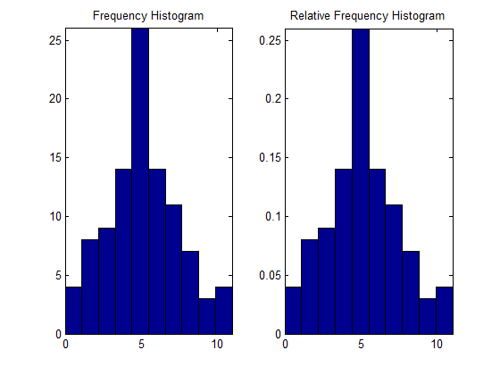
In manufacturing the variation in measurement in processes tend to fall into a normal distribution, for example, the dimensions of parts.

However, an article published in Fortune stated that "of the 58 large companies that have announce Six Sigma programs, 91 percent have trailed the S&P 500 since". The analysis is that, while six sigma is good what it is at, which is "fixing an existing process", it does not help in coming up with new products or disruptive technologies.

Seven Habits

Well, another beautiful "n things" I can recall of is "Seven Habits" from "The Seven Habits of Highly Effective People", a book written by Stephen R. Covey. It is a very good concept of improving oneself (and solving personal problems). It starts off with the concepts of maturity stages; Dependence, Independence and Interdependence.


Beginning with "dependence", without personal development, we will stuck here. People at this stage are inclined to deflect blame and shirk responsibily ("It's not my fault"). From here, there are three habits for self mastery.

Habit 1: Be Proactive
Habit 2: Begin with the End in Mind
Habit 3: Put First Things First

Once one achieves self mastery (self-reliant, independence, take responsibility for one's actions), the next three are to do with interdependence.

Habit 4: Think Win/Win
Habit 5: Seek First to Understand, then to be Understood
Habit 6: Synergize

That this stage (interdependence), we need other people to accomplish our goals (two heads can be much better than one).

And the last habit (renewal)
Habit 7: Sharpen the Saw

Again, there are nice pictures illustrating "seven habits" all over the internet.

I am very pleased to see the Habit 3 here. I knew about the "Covey's Quadrant" time management before, from Randy Pausch's The last lecture. Let me put the 4-quadrant picture here.

Things that we must do can be classified according to two issues "important" and "urgent". We have no problem putting I "important"-"urgent" as the first priority and IV "not important"-"not urgent" as the last priority, but what about II and III ?

It turns out that many people tend to pic III over II (because it is urgent) but this model emphasizes that we need to aim to spend our time in quadrant II. If we don't do II, we will not have the idea of what is important and we will be easily diverted into responding to the urgent instead. What more is, because II is important, in time it will become I.

refs: here and here and here (in thai)

Six Thinking Hats

I was watching TV this afternoon and was impressed by an interview of Edward de Bono. Yes, many of you may already know him, but I did not. He is the creator of "Six thinking Hats" concept. To me, it is a great tool for creative thinking (lateral thinking, think outside of the box). It let us analyze the topic in six different ways. I dug some more information from google images and some of them are selected here.

The benefits of Six Hats I understand now are:
1. Reduce the time of meeting. I have seen so many failed meetings where people talk and talk and they are going no where. Usually, one man talk proposes about a thing, and is interrupted by another man. The interruption might be comments, arguments, showing off that "I am better than you", etc. "Six hats" force everyone to think in parallel by wearing the same hat at the same time.
2. Explore every aspect of an idea (full-spectrum thinking).
3. Separating ego, Improving thinking, questioning, and communicating.

The order of hats depends on the situation. Here is a typical 6 hats workshop.
Step 1: Present the facts of the case ( White Hat))
Step 2: Generate ideas on how the case could be handled (Green Hat)
Step 3: Evaluate the merits of the ideas – List the benefits (Yellow Hat), List the drawbacks (Black Hat)
Step 4: Get everybody’s gut feelings about the alternatives (Red Hat)
Step 5: Summarize and adjourn the meeting (Blue Hat)

In addition to the application of six hats in brain storming workshop, I think it is great for improving individual thinking too. 

refs: Six Thinking Hats, more, even more

Adaptive Mixtures

In finite mixture model approximation, we need to specify the number of mixtures beforehand. We might try to explore the distribution by our eyes. What could be better is the procedure that can get this number automatically. Yes, there is such a procedure. It is called "Adaptive Mixtures". [ Priebe, 1994]

Consider the follow model of three mixtures:

\[f(x) = 0.3\phi (x, - 3,1) + 0.3\phi (x,0,1) + 0.4\phi (x,2,0.5)\]

The data generated from the model is shown as a histogram and distribution plot below.

The following matlab code analyzes the data and gives out the calculated mixtures.

maxterms = 10;

[pihat,muhat,varhat]=csadpmix(data,maxterms);

We can see the result mixtures by:

figure;

csdfplot(muhat,varhat,pihat,min(data),max(data));

axis tight;

It is clear from the above figure that the generated mixtures has 9 terms!. This is normal for adaptive mixtures procedure. The distribution of these mixtures is shown below (it should be similar to the distribution of the original).

Generating Random Variables from a Finite Mixture Model

We can use the finite mixture model to generate more random numbers estimated from the model. For example, using the geyser data:

load(geyser);

hist(geyser,20);

Computational Statistics Toolbox has the csfinmix() function for estimating the finite mixture model. Thus:

>> [p,mu,var]=csfinmix(geyser',[50,80],[1 1],[0.5 0.5],100,1e-5)

p =
    0.3076    0.6924

mu =
   54.2027   80.3603

var =
   24.5223   56.3646

We can use this model to generate more samples, let's try 500 more of them:

n=500;

r = rand(1,n);

ind1 = find(r <= p(1));

ind2 = find(r > p(1));

x(ind2)=normrnd(mu(2),sqrt(var(2)),size(ind2));

x(ind1)=normrnd(mu(1),sqrt(var(1)),size(ind1));

figure;

hist(x,20);

Compare the below figure to the figure above.

Expectation-Maximization (EM) for Finite Mixture Parameters Estimation

EM is a method for optimizing likelihood functions. It is good for situation where data might be missing or when other optimization methods fail.

EM needs some initial guessing for its operations. In this case, we must tell it the number of terms c in the mixture. Plus, we must also guess the initial parameters for each mixture component.

For example, consider this artificial two-term mixture data centered (means) at (-2,2) and (2,0) The covariance of each component is identity (var=1).

EM method consists of two steps. The Expectation step find posterior probability using the data points given the guess parameters of the mixtures (mixing coefficient, means and variances). The Maximization step finds the update mixing coefficient, new means and new variances. These two steps will be iterated until the maximum of errors of any three of them falls below a tolerant limit.

The initial parameters are:

c=2;

[n,d]=size(data); % n=# points, d=# dimension

tol=0.00001;      % each column represents a mean

max_it=100;

%initial guess

mu(:,1)=[-1 -1]';

mu(:,2)=[1 1]';

mix_cof = [0.2 0.8];

var_mat(:,:,1)=eye(d);

var_mat(:,:,2)=eye(d);

The MATLAB code for this task is quite long. Please refer to Example 9.11 of Martinez & Martinez 2008

The final output is:

converge after 39 iterations

p1 = 0.517600, p2 =0.482400

u=

   -2.1795    1.9905

    1.9790   -0.0184

var=

(:,:,1) =

    1.2498   -0.0522

   -0.0522    0.6819

(:,:,2) =

    0.7199   -0.0055

   -0.0055    1.0255

dF Plot

A good approach to visualize parameters for finite mixtures is proposed by Priebe, et al. 1994 and later on extended by many authors. Each component is represented by a circle (or ellipse or ellipsoids) centered at the mean $\mu _i$, and the mixing coefficient $p_i$. The circle size is indicated by its standard deviation.

MATLAB does not have a built-in dF Plot. However we are lucky that we can use the "csdfplot()" function from "Computational Statistics Toolbox" (Martinez & Martinez).

For example for univariate case:

pis = [0.3 0.6 0.4];  % mixing coefficients
mus = [-3 0 2]        % means
vars= [1 1.5 0.5];    % variances
csdfplot(mus,vars,pis,-5,5);

For bivariate case, the variances become a covariance matrix, for example:

given  p = (0.5,0.3,0.2), mu = ((-1,1),(1,1),(5,6)) and vars=((1 0;0 1),((0.5 0; 0 0.5),(1 0.5; 0.5 1))

pis = [0.3 0.6 0.4];
mus = [-3 0 2;-1 1 6];
vars = zeros(2,2,3);
vars(:,:,1)=[1 0; 0 1];     % eye(2)
vars(:,:,2)=[0.5 0; 0 0.5]; % eye(2)*0.5
vars(:,:,3)=[1 0.5; 0.5 1];
figure;
csdfplot(mus,vars,pis);

 
 

Univariate Finite Mixture

Like kernel density estimation (KDE), Finite Mixture (FM) is useful for estimating probability density funciton (PDF). However, unlike KDE, where the bandwidth parameter h is crucial and all of the sample points need to be kept for each evaluation of x, FM needs to take care mainly the number of mixtures and their weights:
$f(x) = \sum\limits_{i = 1}^c {{p_i}g(x;{\theta _i})} $
where $p_i$ represents the weight or mixing coefficient for the i-th term and $g(x;{\theta_i)}$ denotes a probability density, with parameters represented by the vector $\theta_i$

Beware: $p_1+...+p_c = 1$ and $p_i > 0$ and typically comparing to KDE, $c \ll n$


For example,  the model consists of three normal pdf  is
$f(x)=0.4 \phi(x;-3,1)+0.2 \phi(x;0,1)+0.4\phi(x;2,1.5)$

It can be shown by the following MATLAB code:

% finite mixture model
x=linspace(-8,9);
coeff = [0.4 0.2 0.4];
mus = [-3 0 4];
vars = [1 1 1.5];
fhat=zeros(size(x));
for i=1:length(mus) % n terms
    fhat=fhat+coeff(i)*normpdf(x,mus(i),vars(i));
end
plot(x,fhat);

Kernel Density Estimation

Nonparametric probability density estimation can be done using kernel estimators. For a simple univariate case, the kernel estimator is given by:
\[ {\mathop f\limits ^\wedge} _{Ker} (x) = \frac{1}{{nh}}\sum\limits_{i = 1}^n {K(\frac{{x - {X_i}}}{h})} \]
where the function K(t) is call a kernel ($\int {K(t)dt = 1} $).
If we define $ {K_h}(t) = K(t/h)/h$, then
\[ {\mathop f\limits ^\wedge} _{Ker} (x) = \frac{1}{{n}}\sum\limits_{i = 1}^n {K({x - {X_i}})} \]
The smoothing parameter h is called window width, or bandwidth and 1/h is called weight.  A small h yields rough curve while large h yields smooth curve.

The choice of h by Silverman [1986] is $1.06(\sigma){n^{ - 1/5}}$ or $0.786(IQR){n^{ - 1/5}}$ whatever is smaller.

For example, using normal kernel $ K(t) = \frac{1}{{\sqrt {2\pi } }}\exp \left\{ {\frac{{ - {t^2}}}{2}} \right\} $, the following MATLAB code illustrates a kernel density estimation for n=10.

n=10;
kCenter=randn(1,n);
x=linspace(-5,5,100);
fhat=zeros(size(x));
h=1.06*n^(-1/5);
figure;
hold on;
for i=1:n
    f=exp(-((x-kCenter(i))/h).^2/2)/...
      (sqrt(2*pi)*h) /n;
    plot(x,f);
    fhat = fhat + f;
end
plot(x,fhat,'r');
hold off;

The area under the density should be unity. This can be checked by the command:

>> sum(fhat*(x(2)-x(1)))

ans =

    1.0000

Matlab already has the built-in function ksdensity() for the same purpose. 

The method the kernel density estimation here is known as "Parzen Window" method.
ref:  Kernel Density Estimation

Singular Value Decomposition (SVD), Covariance and Correlation Coefficients

SVD

The MATLAB code for SVD is define as:

[u,s,v]=svd(x)

if x is m by n then
u is mxm
s is mxn
v is nxn

x = u*s*v'
u*u' = I 
v*v' = I

Therefore, u and v are orthogonal matrix
ref: svd

Covariance
Matlab function:  cov()
Example: The distribution of a random vector X of bivariate normal distribution is
\[X \sim N(\mu ,\Sigma )\]
where $\rho$ is the correlation between x and y, and the mean and covariance matrix are
\[\mu= \left( {\begin{array}{*{20}{c}}{{\mu _x}}\\{{\mu _y}}\\\end{array}} \right),\;\;\;\;\;\;\Sigma=\left( {\begin{array}{*{20}{c}}{\sigma _x^2} & {\rho {\sigma _x}{\sigma_y}}\\{\rho {\sigma _x}{\sigma _y}} & {\sigma _y^2}\\\end{array}} \right)\]
ref: Covariance Matrix


Correlation Coefficients are derived from covariances

\[r_{xy}=\frac{Cov(x,y)}{{\sigma_x}{\sigma_y}}\]


Matlab function: corrcoef()


ref: Correlation Coefficients
(This post is unfinished, I'll come back later)

Variance of Sample Means

I was always curious and try to understand what does it mean by \[Var(\overline X ) = \frac{{{\sigma ^2}}}{n}\]
My simple MATLAB script can show that if we take 100 samples and compute the mean of them, then do it again 1000 times:

>> dat=poissrnd(5,100,1000);
>> meandat=mean(dat);

the variance of their means are:

>> var(meandat)

ans =

    0.0506

and if we take the variance of all samples (100 x 1000), divide by sample size (100), we got:

>> var(dat(:))/100

ans =

    0.0502

These two numbers are very close!

Glyph Plot, Andrews Plot and Parallel Coordinates Plot

For multidimentional data (multivariate), which means data that has many attributes, visualizing data using these techniques might be useful. The input is a matrix where rows are observations (samples) and columns are variables (attributes).

GlyphPlot displays the data in flower-like icons, sometimes it is slightly different and called “starplot”, “roseplot” or “spiderplot”. For example:

>>load cereal;
>>glyphplot(cereal);

MATLAB glyphplot can show in glyph in Chernoff's “face” style too.

>>glyphplot(cereal,’glyph’,’face’);

Andrews Curves transform each observation into a function f(t) and plot the curve. It is useful in grouping the data.

>> load fisheriris
>> andrewsplot(meas,'group', species);

Parallel Coordinates Plot is similar to Andrews Curves but without the transformation.

>> labs = {'Sepal Length','Sepal Width','Petal Length','Petal Width'};
>> parallelcoords(meas, 'group',species);

More on visualizing multivariate data.

Basic Tools for Exploratory Data Analysis

In Exploratory Data Analysis (EDA), there are several basic tools that might be useful. For example, histogram, Q-Q Plot, Boxplot and Scatterplot Matrix.

Histogram can be plotted using MATLAB hist() function, however if we want it to be a probability mass function, we can simply make a relative frequency histogram, i.e.:

data = poissrnd(5,1,100);

[n,x]=hist(data);

subplot(1,2,1);

bar(x,n,1); axis tight;

title('Frequency Histogram')

subplot(1,2,2);

bar(x,n/sum(n),1); axis tight;

title('Relative Frequency Histogram');

Q-Q Plot is used to compare quartiles of two distributions. If the two distributions are the same we would expect the Q-Q plot to produce a straight line.

Another type of plot related to Q-Q Plot is “Probability Plot”, which can be used to compare the plot of the data to a standard probability distribution.

data2 = randn(1,75);

subplot(1,2,1);

qqplot(data,data2);

subplot(1,2,2);

probplot('normal',data);

Boxplot is another visualized technique to represent the distribution of the data. The lower and upper edge of the box is the 1st and 3rd percentile, therefore the height of the box is called "InterQuartile Range (IQR)". Moreover, it can show the most extreme values as the lower and upper limit (wisker), plus the outliers.

load carsmall

boxplot(MPG,Origin);

Scaterplot Matrix is a way to display multi-dimensional data by looking at 2D scatterplots of all possible pairs of variables. In MATLAB, we can use the plotmatrix() function.

load iris

plotmatrix(setosa);

title('Iris Setosa');